Optimal Streaming Histograms

How can you create a bucketing algorithm for an arbitrary dataset you don’t know in advance?

We get a constant stream of numerical data from our customers. We’re not sure what the range of this data might be or how many orders of magnitude it may span. The distribution of the data is constantly changing as new data is added.

It’s not feasible to keep track of all of these distinct values, both on the database end and for data visualization — we need to sort it into buckets. How can we decide on a reasonable bucketing algorithm for histogramming solution boundaries for all of these constantly changing datasets?

Basically, this boils down to 2 key requirements. Our bucketing algorithm needs to generate bucket boundaries that:

1. are useful & reasonable for any range of data

2. remain useful even if the distribution of the data changes

We went through a few iterations of bucketing algorithms before we landed on our current solution.

Technique #1: Save the first 1000 distinct values, and then make evenly spaced buckets.

This is the most naive way to bucket. We made 50 evenly spaced buckets across the range of the first 1000 values, and included 1 bucket for everything below that range, and 1 bucket for everything above it.

Problems with Technique #1:

1. Resolution

Say you have a highly skewed distribution of values with a long tail:

With evenly spaced buckets (dotted lines – in this example, 10 buckets), you lose resolution exactly where the majority of your values are.

2. Fixed buckets

If the distribution changes over time, the chosen buckets won’t be applicable anymore. We did our best to get around this issue by re-bucketing each day.

3. Strange (arbitrary) spacing

With even spacing, our buckets each had a width of: [range of values]/50. This resulted in weird bucket ranges that didn’t correspond to anything meaningful.

Technique #2: Iteratively merge the closest values into buckets

We tried Technique #2 to solve the resolution problem. We took the first 1000 distinct values and merged the 2 values that were closest together into 1 bucket. We then did this over and over again until we had 50 buckets.

Problems with Technique #2:

Although this made resolution better, it made the strange spacing problem even worse. Not only did bucket ranges seem arbitrary, but all of the bins were of different widths. This was especially problematic when visualizing the data in a histogram.

Let’s illustrate with a simple example. We have this list of 20 numbers, and we want to put them in 10 buckets:

3, 6, 7, 8, 13, 20, 23, 28, 31, 42, 45, 50, 63, 70, 74, 85, 88 93, 95, 98

We run the merging algorithm and end up with these bins:

The buckets are all of varying width, which makes the x-axis deceptive. And again, this technique runs into the problem of having to update the bucketing scheme whenever the data’s distribution changes.

Interlude: the Equal Width vs. Equal Height Conflict

When deciding on bucket size, there’s a constant struggle between equal height buckets and equal width buckets. Technique #1 had equal width buckets, which are nice and neat, but ran into the resolution problem. Technique #2, which iteratively merged the closest distinct values into buckets, was an attempt at equal height buckets — ie, buckets that each held about the same number of values, no matter the distribution of those values. However, we got weird spacing issues.

This brings us to Technique #3:

Technique #3: V-optimal bucketing

V-optimal histograms try to strike a balance between optimizing for equal height and equal width buckets. The idea is to minimize the cumulative weighted variance, which is defined as:

where J is the number of buckets, nj is the number of items in the _j_th bin, and Vj is the variance between values in the _j_th bin. V-optimal histograms are better at estimating bucket contents than either equal width or equal height histograms.

Problems with Technique #3:

The key disadvantage with this technique is that choosing the optimal bucket boundaries gets very complex as the range of values and number of buckets increases. This also means it’s difficult to update (again, the problem of fixed buckets as distributions change over time).

We never actually implemented V-optimal bucketing, but we did consider it. Ultimately, we decided on technique #4:

Technique #4: Pre-create buckets on a logarithmic scale

For a given range of values, we used a pre-determined bucket size: 10% increments for every order of magnitude. The table below shows our bucket sizes for a given range of values:

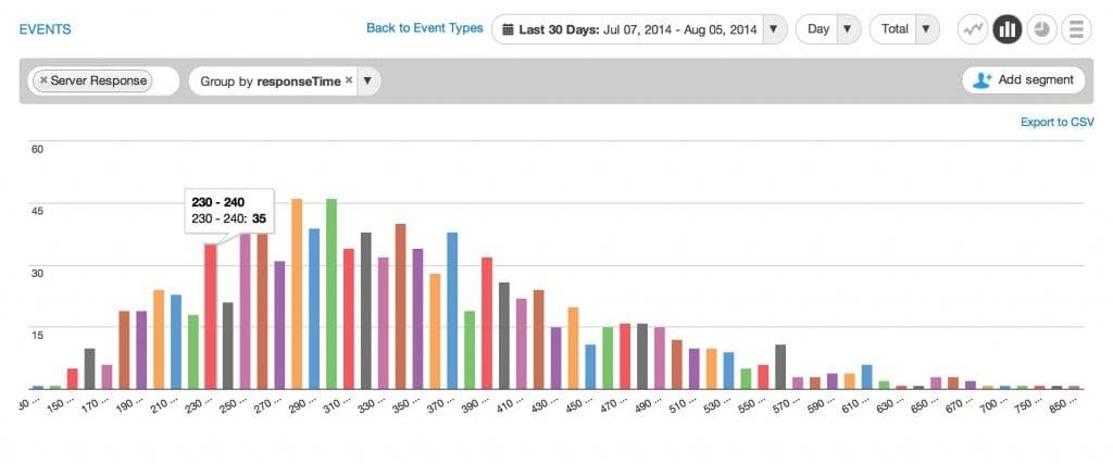
Here’s an example from the Amplitude dashboard. We’re looking at the responseTime property of an event called Server Response. Since the data falls in the 100-1000 range, the buckets are in increments of 10:

Problems that Technique #4 SOLVES:

1. Resolution: This method ensures that no matter what a value is, the range of the bucket will be within 10% of the true value, or two significant figures. That’s plenty for almost all histograming needs.

2. Fixed width buckets: With this method, having buckets of fixed width is a viable option. We no longer have to worry about adjusting the buckets every time the distribution changes. This bucketing scheme should work for a variety of data set types, and works across any range of values.

3. Strange spacing: With these pre-determined buckets that can be applied to any range of values, we no longer have weird buckets like 63.47 to 84.19. Everything is nice and neat.

Admittedly, this method is still not ideal for data visualization if your data spans several orders of magnitude. Buckets have different widths at different orders of magnitude, but at least the width progresses in a way that’s predictable and is fixable in a visualization.

Ultimately, we decided on this bucketing algorithm because it allows us to efficiently collect continuous value data and organize it with a minimal loss of resolution in the information. It meets our 2 key requirements: being useful for any range of data and remaining useful even if the distribution of the data changes.

Thoughts? Join the discussion on Hacker News.